A Practical Approach to Understanding CRE Portfolio Risk, Diversification, and the Impact of Leverage: A Case Study
For decades, investors have evaluated both risk and return in real estate investments. While there is a range of well-understood return metrics (internal rate of return [IRR], total returns, etc.), risk metrics are often confined to textbooks and university finance faculties. Investors know intuitively that spreading real estate investments across sectors and markets tends to increase diversification and reduce portfolio risk - but by how much? Investors also know that leverage tends to increase expected returns while increasing risk - but again, by how much? At what point does the additional risk associated with increasing leverage outweigh the benefits of increased returns?
This article shows that, by carefully modelling risk at the property and portfolio levels, with and without leverage, we can quantify commercial real estate (CRE) investment risk and then construct portfolios that reduce risk, increase diversification, and optimize leverage. To do so, we may also have to challenge the use of Sharpe ratios as the go-to risk metric for CRE investors.
The Case Study Portfolio
The analysis in this article is based on the direct Canadian real estate holdings of OPTrust. OPTrust invests and manages one of Canada's largest public-sector pension funds and administers the Ontario Public Service Employees Union (OPSEU) Pension Plan, a defined benefit plan with almost 95,000 members and retirees. OPTrust's Member-Driven Investing strategy is focused on maintaining the fully funded status of the plan, seeking to deliver sufficient investment returns without taking on excess investment risk. To deliver on its mandate, OPTrust has developed risk-modelling tools and, in the case of its real estate investments, this has led to a collaboration with Radley Associates, an independent firm dedicated to the development of simulation-based analytics for the commercial real estate industry.
The case study investor used a Monte Carlo simulation model to project all likely investment outcomes for each property and portfolio in 10,000 scenarios. From the statistical distribution of these IRRs, the average IRR (expected return) and standard deviation of IRRs (volatility or risk) were calculated. The rent-roll data and property-level assumptions for each property were based on the investor's latest appraisals.
Case Study Results
OPTrust's real estate portfolio primarily comprises income-producing office, industrial, multifamily residential, and retail properties. Each property in the portfolio was analyzed individually (without leverage), and the expected ten-year IRR and standard deviation of each property were recorded. Thereafter, the weighted average IRR and standard deviation were calculated for the entire portfolio ("Weighted Average Portfolio" in Exhibit 1).
| IRR | Volatility | |
|---|---|---|
| Weighted Average Portfolio | 6.81% | 3.32% |
But what about diversification? Taking a weighted average of the individual IRRs and volatilities ignores the impact of diversification on the portfolio. In reality, many of the factors that affect performance are largely uncorrelated. For example, while Canadian office and property market cap rates may be highly correlated, tenants still vacate and renew in largely uncorrelated ways, so overall property performance can be diversified across the portfolio. By using a Monte Carlo simulation, the combined cash flows of all properties across each scenario were analyzed so that a true portfolio distribution could be calculated across the portfolio ("True Portfolio" in Exhibit 2). The difference between the true portfolio and the weighted average portfolio results is the measure of portfolio diversification.
| IRR | Volatility | |
|---|---|---|
| Weighted Average Portfolio | 6.81% | 3.32% |
| True Portfolio | 7.11% | 2.22% |
| Benefit of Diversification (True − Weighted) | 0.30% | −1.10% |
The true portfolio has 110 basis points (bps) less volatility than the weighted average volatility of the individual properties, and this is the measure of the portfolio's diversification benefit. The portfolio also generates an improvement to the mean return of 30 bps - a result that is consistent with theory but rarely calculated.
This result has two practical uses for investors. First, investors can look at individual properties (either existing or under consideration for acquisition) and determine whether they improve or reduce the diversification of the overall portfolio. Second, quantifying the diversification benefit can be used to communicate to stakeholders how much value the portfolio is adding in terms of volatility (or risk) reduction. Investment managers can now talk not only about higher returns but also about lower risk.
The Risk-Return Space
How can we tell if the overall portfolio result - in terms of risk and return - is a good one or not? How do we compare it with other asset classes? By plotting the risk and return of the CRE portfolio (with and without diversification) in the risk-return space, comparisons can be made with alternative asset classes (Exhibit 3). In this case, returns of ten-year government bonds (return of 2.30% with no volatility) and the total returns of an investment in Canadian stocks held for ten years (return of 6.59% with volatility of 3.20%) can be analyzed. A combined holding can generate a risk-return profile anywhere along the stock-bond line (shown in gray).
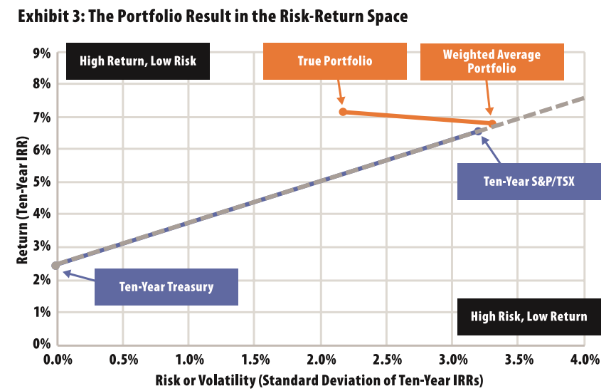
The (unleveraged) Canadian CRE portfolio generates an expected, weighted average, or prediversification, risk-return profile very similar to an equity portfolio. But once diversification is recognized in the CRE portfolio, the true risk-return profile of the portfolio is considerably better than any combination of stocks and government bonds could achieve.
Leverage
The analysis above reflects the returns of the portfolio when each property is simulated assuming no leverage. In reality, the investor utilizes a moderate level of fixed or floating-rate leverage on some of its properties. But does leverage improve the portfolio performance in the risk-return space? Would more or less leverage move the portfolio farther above the stock-bond portfolio line (all else being equal)?
The simulation analysis was run again, but this time including the impact of debt costs and repayments on the cash flows and exit values of the true portfolio.
Sharpe Ratio and Leverage
Doesn't financial theory say that you can't improve the Sharpe ratio by adding leverage? In a simple, single-property model with normal distributions of IRRs and no correlations, this may be true, but we know that CRE returns are skewed and correlated in real life, so what is happening?
The comparison of the weighted average portfolio result with and without leverage is instructive. The comparison below reflects the impact of leverage on each individual property without including the impact of diversification.
| IRR | Volatility | |
|---|---|---|
| Unleveraged | 6.81% | 3.32% |
| Actual Leverage | 7.79% | 4.38% |
| Impact of Leverage (Actual Leverage − Unleveraged) | 0.98% | 1.06% |
In the analysis (the wrong one in our view), the leverage increases the returns by 98 bps, but the increase in volatility is higher, at 106 bps. This is because the analysis does not reflect the diversification of leverage risk: adverse or beneficial movements in debt costs (whether of floating-rate interest costs or the uncertain costs of refinancing) are not fully correlated with property performance - in particular, cap rate risk. As a result, increases in volatility in each property may be offset by diversification at the portfolio level - and this is indeed the case. This finding may have important implications for leverage strategy; for example, leverage of varying terms and structures at the property level may create higher portfolio diversification than a single leverage instrument at the fund or portfolio level.
| IRR | Volatility | |
|---|---|---|
| Unleveraged | 7.11% | 2.22% |
| Actual Leverage | 8.34% | 2.80% |
| Impact of Leverage (Actual Leverage − Unleveraged) | 1.23% | 0.58% |
In this portfolio, the volatility is increased by leverage, as expected, but by only 58 bps, while the expected IRR is increased by 123 bps (Exhibit 4). The increase in return far outweighs the increase in volatility - on the face of it, a successful leverage strategy.
The Risk-Return Space Again
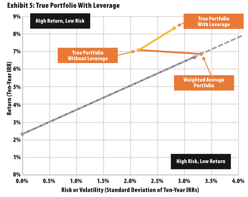
Now that leverage has been added to the analysis, the true portfolio result can be calculated. True portfolio results reflect diversification effects. Exhibit 5 shows that leverage has added more return to the unleveraged portfolio than it has added volatility relative to the gray stock-bond line. The resulting true portfolio return and risk metrics are a return of 8.34% (ten-year IRR) and volatility/risk of 2.80% (standard deviation). This level is superior, on average, to any (unleveraged) combination of stocks and government bonds. But can we be sure that the increase in volatility of 58 bps is more than justified by the increase in returns of 123 bps?
The gradient of the stock-bond line indicates the average investor's trade-off of ten-year IRR and ten-year volatility. In today's markets, Canadian investors will trade off about 1.35% of return to reduce volatility by 1%. On this basis, Exhibit 5 shows that the leveraged returns are better than the unleveraged returns.
By trading volatility for return of the leveraged and unleveraged portfolios, the leveraged portfolio can return 4.60% on a "risk-free equivalent basis" and the unleveraged portfolio, 4.16%. Both are better than the risk-free rate (Treasury bond rate), but adjusting for volatility, leverage adds about 44 bps of risk-free equivalent return.
Sharpe and Other Measures of Risk-Adjusted Returns
The Sharpe ratio is often used in finance to compare the risk-adjusted returns of two alternative portfolios. It is defined as the expected return less the risk-free rate all divided by the volatility of returns. In this case, results of the Sharpe ratios of the leveraged and unleveraged (true) portfolio were compared. The higher the Sharpe ratio, the better the risk-adjusted returns.
| IRR | Volatility | Risk-Free Rate | Sharpe Ratio | |
|---|---|---|---|---|
| True Portfolio Unleveraged | 7.11% | 2.22% | 2.31% | 2.16 |
| True Portfolio With Leverage | 8.34% | 2.80% | 2.31% | 2.15 |
| IRR | Volatility | Risk-Free Rate | Sharpe Ratio | |
|---|---|---|---|---|
| Portfolio A | 4.00% | 0.10% | 2.31% | 16.9 |
| Portfolio B | 8.00% | 0.50% | 2.31% | 11.4 |
It appears then, using Sharpe ratios, that the unleveraged portfolio is (marginally) better than the leveraged portfolio. In fact, Sharpe ratios for portfolios with financing costs that are higher than the risk-free rate will always be lower than for unleveraged portfolios. Strict users of the Sharpe ratio would therefore never add leverage to portfolios. But is this the right conclusion?
We argue that the Sharpe ratio is an incomplete measure and that there are better ways of looking at these results in practice. Imagine that there are two portfolios, A and B, with the following characteristics:
Relying on only the Sharpe ratio, Portfolio A is preferable to Portfolio B as it has a higher Sharpe ratio, but a look at the graphic representation below may lead to a different conclusion.

The Sharpe ratio measures the gradient of the line between the riskless Treasury bond position and Portfolios A and B. On this measure, Portfolio A is preferable to Portfolio B. But the stock-bond risk-return line shows that investors will generally sacrifice about 1.35% of return for a 1% reduction in volatility (the gradient of the gray line). Using this approach, Portfolio B is much more attractive than Portfolio A, as can be seen graphically by following the dotted lines that are parallel to the gray risk-neutral line from Portfolios A and B to the y-axis. The intersect of the y-axis for Portfolio B is much higher than for Portfolio A.
Optimizing Leverage
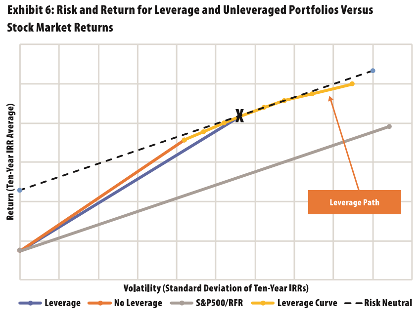
The approach outlined above gives investors a tool to optimize leverage at the portfolio level. The optimal level of leverage will be different for every CRE portfolio depending on its inherent level of diversification, average expected returns, and the cost of available financing, among other factors. Because of the multiple factors involved, there is no single equation that can determine the perfect level of leverage for any portfolio. To optimize the level and type of leverage, alternative debt structures should be modelled at the property and portfolio levels as each debt instrument comes to maturity and financing options present themselves to the investor. However, the simulation approach allows investors to develop a leverage strategy that can be fine-tuned with each financing decision. As the level of leverage increases, financing costs rise (lenders ask for higher margins for higher loan-to-value ratios) and the increasing cost of financing eventually reduces the risk-adjusted benefits of leverage (Exhibit 6).
Conclusions: CRE Investors Care as Much (or More) About Volatility as They Do About Returns
Risk or volatility in real estate portfolios can be calculated using cash-flow simulation. True portfolio-level diversification can be quantified and communicated to stakeholders as the basis of an informed dialogue about risk as well as return, placing CRE investment alongside traditional asset classes, where discussion of volatility alongside returns has long been the norm.
If this case study of OPTrust's real estate portfolio is typical of the industry, CRE investors should be able to transcend the label "alternative investments" and demonstrate that they can also manage portfolios on a quantified risk-adjusted basis. The portfolio in this case study provides roughly 1.1% lower volatility through diversification - worth more than 1.5% in extra returns to an average ten-year investor. Leverage can also be shown to add a further 45 bps in risk-adjusted returns. For OPTrust as a pension management organization, this is a meaningful impact for our members, helping us reach our goal of providing certainty, sustainability, and security in retirement.
Managing portfolio risk and return by calculating the marginal contribution of each property (or proposed property) to the volatility of the portfolio as well as the returns of the portfolio should allow for a more sophisticated approach to portfolio construction. The case study also shows that leverage can add value to a portfolio, on a risk-adjusted basis, when diversification is taken into account and that simulation can provide a practical framework for fine-tuning and optimizing leverage.
Charles Cardozo is Operations Director, Peter Michaels is Head of Methodology, and Howard Radley is Founder and Managing Director of Radley Associates. Robert Douglas is Managing Director, Real Estate Group; Matthew Glick and Umair Raza are Associate Portfolio Managers, Real Estate Group, at OPTrust.
This article has been prepared solely for informational purposes and is not to be construed as investment advice or an offer or a solicitation for the purchase or sale of any financial instrument, property, or investment. It is not intended to provide, and should not be relied on for, tax, legal, or accounting advice. The information contained herein reflects the views of the author(s) at the time the article was prepared and will not be updated or otherwise revised to reflect information that subsequently becomes available or circumstances existing or changes occurring after the date the article was prepared.
- If IRR distributions were normally distributed and noncorrelated, this benefit would be zero. However, in Monte Carlo simulations, which use actual distributions (i.e., non-normal) and where variables are highly correlated, benefits to the mean are generally positive except in cases of high leverage.
- Average ten-year yield for Canadian Treasury bonds for 2018.
- S&P/TSX average total returns and volatility for an investment held for ten years between 1971 and 2018.
- Note that the US stock market performance is more volatile over time than the Canadian stock market.
- Note that total stock market returns also recognize the diversification of the individual stocks that make up the index, so the comparison is valid.
- The simulation model assumes that all leverage is refinanced at term at the prevailing market interest rates in each scenario.
- Randall Zisler and Matthew Zisler, "Rising Interest Rates Will Not Necessarily Increase Cap Rates," PREA Quarterly, Spring 2016, pp. 52–56.
- Some may view the ten-year volatility of 2.80% as unexpectedly low. Models that do not include reversion to mean assumptions tend to show volatility widening with time, but reversion to mean is strongly supported by historical data. Intuitively, we believe this is correct, and while the precise level of reversion to mean is a modelling choice, to ignore it would be to miss a key feature of property values and their relationship to long-term value in advanced economies.
- This trade-off, or cost of volatility, is calculated as (stock market returns − risk-free rate) / stock market volatility. The precise quantity (calculated as 1.35 here) may vary by market and over time.
- Realistic levels of correlation between key assumptions (cap rates, vacancy periods, inflation, rental growth rates, etc.) need to be explicitly modelled and managed.
This program was established to encourage and expand active participation in our educational and research initiatives by junior associates within PREA's investor constituency. Once appointed, Fellows make a two-year commitment to attend both PREA conferences and the PREA Institute as well as engage in our committee activities and Affinity Group program. Eligible individuals are encouraged to apply for the program directly. However, supervisors may also nominate eligible individuals who work within their organizations. For more information, visit the PREA website at www.prea.org/awards/koza.